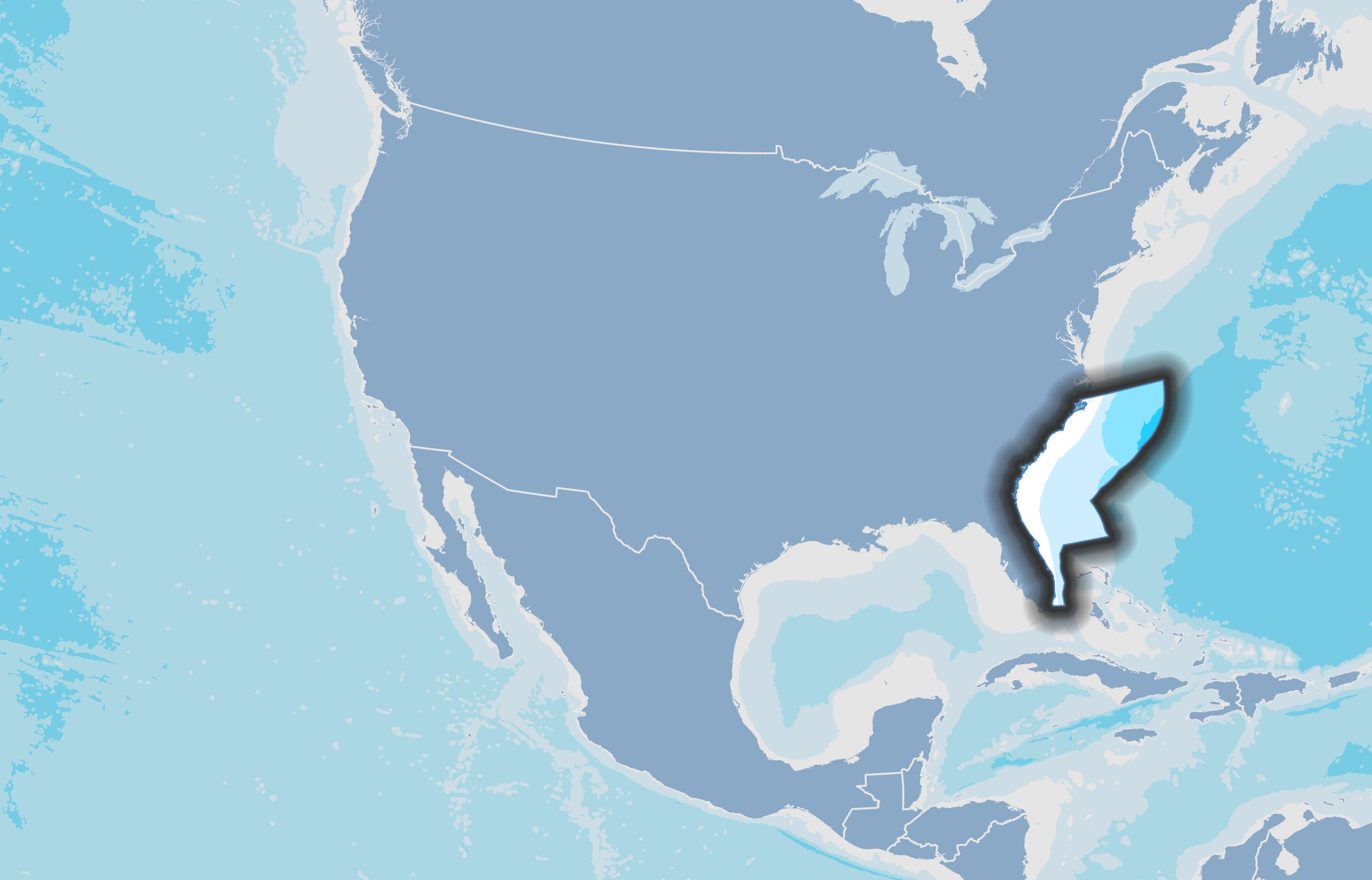
Spanning the area from North Carolina to Florida, the Southeast contains over 18,000 miles of coastline. With extensive riverine, estuarine, marsh, barrier island, mangrove, and coral reef systems, the Southeast has the largest wetland acreage and coral reef track in the contiguous United States, and one of the world’s largest shallow water coral reef ecosystems.
A diversity of life is supported in this region, including 18 protected marine species. The Southeast region provides the only known calving grounds for the highly endangered North Atlantic Right Whale. Bottlenose dolphins, sea turtles, diverse coral, sawfish, Bryde's whales, manta rays, and shortnose and Atlantic sturgeon also reside in this region.
The Gulf Stream is an important influence on biological, chemical, and physical characteristics of the region. Natural hazards include thunderstorms and tornadoes; floods and debris flows; drought and wildfires; winter storms; ground subsidence; coastal erosion; and hurricanes. Coastal hazards are major concerns, since over one-third of the population resides in coastal counties and over 4 million people live in flood hazard areas.
This region contributes more than 10% of the total U.S. economy, with coastal recreation, tourism, recreation, transportation, and shipping being major contributors to the regional economy. Home to one of the largest concentrations of saltwater recreational fishing in America, the Southeastern United States generates more than $15 billion annually for more than 4.5 million fishermen. The region has over 35 ports and terminals that service cargo and passenger ships, including some of the country’s largest and fastest growing container ports.
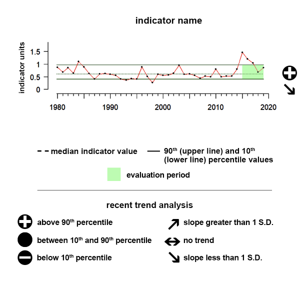
Understanding the Time series plots
Time series plots show the changes in each indicator as a function of time, over the period 1980-present. Each plot also shows horizontal lines that indicate the median (middle) value of that indicator, as well as the 10th and 90th percentiles, each calculated for the entire period of measurement. Time series plots were only developed for datasets with at least 10 years of data. Two symbols located to the right of each plot describe how recent values of an indicator compare against the overall series. A black circle indicates whether the indicator values over the last five years are on average above the series 90th percentile (plus sign), below the 10th percentile (minus sign), or between those two values (solid circle). Beneath that an arrow reflects the trend of the indicator over the last five years; an increase or decrease greater than one standard deviation is reflected in upward or downward arrows respectively, while a change of less than one standard deviation is recorded by a left-right arrow.
North Atlantic Oscillation (NAO)
During the last five years, the NAO indicator shows no significant trend but has remained largely in the negative phase.
Values correspond to Index scores
Description of time series:
Positive NAO values mean significantly warmer winters over much of the eastern U.S. and northern Europe and negative NAO values can mean cold winter outbreaks and heavy snowstorms. During the last five years, the NAO indicator shows no significant trend but has remained largely in the negative phase.
Description of North Atlantic Oscillation (NAO):
The North Atlantic Oscillation (NAO) Index measures the relative strengths and positions of a permanent low-pressure system over Iceland (the Icelandic Low) and a permanent high-pressure system over the Azores (the Azores High). When the index is positive (NAO+) significantly warmer winters can occur over much of the eastern U.S. This prevents nutrient-rich upwelling, which reduces productivity. When the NAO index is negative, the upper central and eastern portions of the United States can incur winter cold outbreaks and heavy snowstorms. This climate condition impacts people and ecosystems across the globe and each of the indicators presented here. Interactions between the ocean and atmosphere alter weather around the world and can result in severe storms or mild weather, drought, or flooding. Beyond “just” influencing the weather and ocean conditions, these changes can produce secondary results that influence food supplies and prices, forest fires and flooding, and create additional economic and political consequences.
Data:
Climate indicator data was accessed from the NOAA NCEI (https://www.NCEI.noaa.gov/teleconnections/nao). The data plotted are unitless anomalies and averaged across a given region.
Atlantic Multidecadal Oscillation
During the last five years, the AMO has largely been in a positive phase, and continues to trend upward.
Values correspond to Index scores
Description of time series:
Positive AMO values indicate the warm phase, during which surface waters in the North Atlantic Ocean are warmer than average, and negative AMO values indicate the cold phase, during which surface waters in the North Atlantic Ocean are cooler than average. During the last five years, the AMO has largely been in a positive phase, and continues to trend upward.
Description of Atlantic Multidecadal Oscillation (AMO):
The Atlantic Multidecadal Oscillation is a series of long-duration changes in the North Atlantic sea surface temperature, with cool and warm phases that may last for 20-40 years. Most of the Atlantic between the equator and Greenland changes in unison. Some areas of the North Pacific also seem to be affected. This broadscale climate condition affects air temperatures and rainfall over much of the Northern Hemisphere. It is also related to major droughts in the Midwest and the Southwest of the U.S. In the warm phase, these droughts tend to be more frequent and/or severe. Vice-versa for the cold phase. During the warm phases the number of tropical storms that mature into severe hurricanes is much greater than during cool phases. Despite the association of AMO with multiple weather and climate impacts, recent scientific debate has questioned whether this indicator is a natural climate variation, like the other climate indicators presented here, or a response of the climate system to human-caused climate change. Whether natural or a result of human-caused climate change, AMO is a useful feature for tracking large-scale weather and climate events. This climate condition impacts people and ecosystems across the globe and each of the indicators presented here. Interactions between the ocean and atmosphere alter weather around the world and can result in severe storms or mild weather, drought, or flooding. Beyond “just” influencing the weather and ocean conditions, these changes can produce secondary results that influence food supplies and prices, forest fires and flooding, and create additional economic and political consequences
Data Background:
Climate indicator data was accessed from NOAA’s Earth Systems Research Laboratory (https://www.esrl.noaa.gov/psd/data/timeseries/AMO/). The data plotted are unitless anomalies and averaged across a given region
Southeast SST
During the last five years there has been no notable trend but values have been above the 90th percentile of all observed data in the time series.
Sea surface temperature is defined as the average temperature of the top few millimeters of the ocean. Sea surface temperature monitoring tells us how the ocean and atmosphere interact, as well as providing fundamental data on the global climate system
Data Interpretation:
Time series: The time series shows the integrated sea surface temperature for the Southeast US region. During the last five years there has been no notable trend but values have been above the 90th percentile of all observed data in the time series.
Indicator and source information:
The SST product used for this analysis is the NOAA Coral Reef Watch CoralTemp v3.1 SST composited monthly (https://coralreefwatch.noaa.gov/product/5km/index_5km_sst.php) accessed from CoastWatch (https://oceanwatch.pifsc.noaa.gov/erddap/griddap/CRW_sst_v3_1_monthly.g…).
Great Lakes SST data were accessed from (https://coastwatch.glerl.noaa.gov/glsea/glsea.html).
The data are plotted in degrees Celsius.
Data background and limitations:
The NOAA Coral Reef Watch (CRW) daily global 5km Sea Surface Temperature (SST) product, also known as CoralTemp, shows the nighttime ocean temperature measured at the surface. The CoralTemp SST data product was developed from two, related reanalysis (reprocessed) SST products and a near real-time SST product. Monthly composites were used for this analysis.
Southeast Sea Level
During the last five years, there has been no trend but values are greater than 90% of all observed data in the time series.
Sea level varies due to the force of gravity, the Earth’s rotation and irregular features on the ocean floor. Other forces affecting sea levels include temperature, wind, ocean currents, tides, and other similar processes.
Description of time series:
The time series shows the relative sea level for this region. During the last five years, there has been no trend but values are greater than 90% of all observed data in the time series.
Indicator and source information:
NOAA monitors sea levels using tide stations and satellite laser altimeters. Tide stations around the globe tell us what is happening at local levels, while satellite measurements provide us with the average height of the entire ocean. Taken together, data from these sources are fed into models that tell us how our ocean sea levels are changing over time. For this site, data from tide stations around the US were combined to create regionally averaged records of sea-level change since 1980. We present data for all regions.
Data background and limitations:
Sea level data presented here are measurements of relative sea level, water height as compared to nearby land level, from NOAA tide gauges that have >20 years of hourly data served through NOAA’s Center for Operational Oceanographic Products and Services (CO-OPS) Tides and Currents website. These local measurements are regionally averaged by taking the median value of all the qualifying stations within a region. The measurements are in meters and are relative to the year 2000.
Southeast Heatwave Intensity
During the last five years there has been no trend and the five-year average is between the 10th and 90th percentiles of all observed data in the time series.
Values indicate cumulative annual heatwave intensity and duration in a region in degree-days
Description of Time Series: This time series shows the average integrated degree day value for the Southeast region. During the last five years there has been no trend and the five-year average is between the 10th and 90th percentiles of all observed data in the time series.
Indicator Source Information:
The marine heatwave data shown here are calculated by NOAA’s National Centers for Environmental Information using Optimum Interpolation Sea Surface Temperature (OISST) data. The NOAA 1/4° OISST is a long term Climate Data Record that incorporates observations from different platforms (satellites, ships, buoys and Argo floats) into a regular global grid. The dataset is interpolated to fill gaps on the grid and create a spatially complete map of sea surface temperature. Satellite and ship observations are referenced to buoys to compensate for platform differences and sensor biases.
Data Background and Caveats:
Heatwave metrics are calculated using OISST, a product that uses some forms of interpolation to fill data gaps. Heatwaves are defined by Hobday et al., 2016 as distinct events where SST anomaly reaches the 90th percentile in a pixel for at least 5 days, separated out by 3 or more days.
Southeast Heatwave Area
During the last five years there has been no trend and the five-year average is between the 10th and 90th percentiles of all observed data in the time series.
Values indicate monthly percent of an LME area affected by heatwave
Description of Time Series:
This time series shows the monthly heatwave spatial coverage for the Southeast Region. During the last five years there has been no trend and the five-year average is between the 10th and 90th percentiles of all observed data in the time series.
Indicator Source Information:
The marine heatwave data shown here are calculated by NOAA’s National Centers for Environmental Information using Optimum Interpolation Sea Surface Temperature (OISST) data. The NOAA 1/4° OISST is a long term Climate Data Record that incorporates observations from different platforms (satellites, ships, buoys and Argo floats) into a regular global grid. The dataset is interpolated to fill gaps on the grid and create a spatially complete map of sea surface temperature. Satellite and ship observations are referenced to buoys to compensate for platform differences and sensor biases.
Data Background and Caveats:
Heatwave metrics are calculated using OISST, a product that uses some forms of interpolation to fill data gaps. Heatwaves are defined by Hobday et al., 2016 as distinct events where SST anomaly reaches the 90th percentile in a pixel for at least 5 days, separated out by 3 or more days.
Southeast pCO2
Between 2019 and 2024 pCO2 showed no trend but was near the top of the range of historical values.
The pCO2 data shown here as an ecosystem indicator of ocean acidification represent regional monthly averages of these mapped estimates.
Description of Time Series: Between 2019 and 2024 pCO2 showed no trend but was near the top of the range of historical values.
Description of Sea Surface pCO2:
Carbon dioxide (CO2) released from fossil fuel burning and other human activities (also known as “anthropogenic CO2”) not only accumulates in Earth’s atmosphere, but is also absorbed by seawater at the ocean surface. This process represents a double-edged sword for the planet: CO2, which has negative consequences for climate change, is removed from the atmosphere but it also contributes to the acidification of ocean waters, which can harm sea life like corals and crabs. The partial pressure of CO2 in seawater (pCO2) represents the relative amount of CO2 in the water. It is a critical metric for calculating the exchange of CO2 across the air–sea interface and for tracking the effects of anthropogenic carbon on surface ocean chemistry.
Data Source:
Global observations of pCO2 from automated shipboard systems that take in and analyze water while a vessel is moving are aggregated in the Surface Ocean CO2 Atlas (SOCAT; Bakker et al., 2016). These shipboard observations have been combined with data from available observational, model-based, and satellite products (e.g., sea-surface temperature, salinity, and wind speed) to create estimates of surface ocean pCO2 in U.S. Large Marine Ecosystems over multiple decades, using a technique known as machine learning (Sharp et al., 2024). The pCO2 data shown here as an ecosystem indicator of ocean acidification represent regional annual averages of these mapped estimates. Uncertainty in pCO2 is estimated from a data-based validation of the machine-learning algorithms for each Large Marine Ecosystem, scaled by the data coverage in a given month. The complete dataset is available at https://www.ncei.noaa.gov/data/oceans/ncei/ocads/metadata/0287551.html.
Close
Southeast pH
Between 2019 and 2024 pH showed no significant trend and was below historical values.
The pH data shown here as an ecosystem indicator of ocean acidification represent regional monthly averages of these estimates.
Description of Time Series: Between 2019 and 2024 pH showed no significant trend and was below historical values.
Description of Sea Surface pH:
Man-made (or “anthropogenic”) CO2 that is taken up by the ocean influences the chemistry of seawater, resulting in an increase in hydrogen ion concentration of the surface ocean (i.e. a decrease in surface ocean pH). pH can be viewed as a “master variable” in ocean chemistry, controlling acid-base balance in the sea. It is also a common way to quantify ocean acidification: average surface ocean pH has decreased by more than 0.1 units since the beginning of the industrial revolution (Jiang et al., 2023).
Data Source:
Mapped estimates of surface-ocean pCO2 in U.S. Large Marine Ecosystems (LME’s) (Sharp et al., 2024), based on observations from the SOCAT database, have been paired with another key ocean-carbon variable called total alkalinity (TA), estimated from salinity, temperature, and spatial information using algorithms called ESPERs (Carter et al., 2021), to calculate surface ocean pH across the U.S. LME’s. The pH data shown here as an ecosystem indicator of ocean acidification represent regional annual averages of these estimates. Uncertainty in pH is determined by propagating pCO2 and TA uncertainties through calculations, using reasonable estimates of uncertainty in required chemical constants and ancillary variables. The complete dataset is available at https://www.ncei.noaa.gov/data/oceans/ncei/ocads/metadata/0287551.html.
Southeast Aragonite
Between 2019 and 2024 Sea Surface Ωar showed a significant downward trend and was below historical values.
The Ωar data shown here as an ecosystem indicator of ocean acidification represent regional averages of these estimates.
Description of Time Series: Between 2019 and 2024 Sea Surface Ωar showed a significant downward trend and was below historical values.
Description of Sea Surface Ωar:
Many marine animals and plants build shells or other hard parts from the minerals aragonite and calcite, which are forms of the chemical compound calcium carbonate. The chemical building blocks of these minerals are calcium and carbonate ions, which are common constituents of seawater. However, one effect of ocean acidification is to reduce the carbonate ion concentration in seawater, making it more difficult for these minerals to form. The chemical expression that describes the tendency of these minerals to form at equilibrium is called the saturation state of that mineral: higher values support mineral formation, while lower values inhibit mineral formation, or even promote the dissolution of these minerals. We present here saturation-state estimates for the mineral aragonite (Ωar), which is used by many marine organisms including corals, mollusks, and some zooplankton to create hard parts. At 20°C, saturation state of the mineral calcite is about 50% higher than aragonite (Mucci, 1983)
Data Source:
Mapped estimates of surface-ocean pCO2 in U.S. Large Marine Ecosystems (LME’s) (Sharp et al., 2024), based on observations from the SOCAT database, have been paired with another key ocean-carbon variable called total alkalinity (TA), estimated from salinity, temperature, and spatial information using algorithms called ESPERs (Carter et al., 2021), to calculate surface-ocean Ωar across the U.S. LME’s. The Ωar data shown here as an ecosystem indicator of ocean acidification represent regional averages of these estimates. Uncertainty in Ωar is determined by propagating pCO2 and TA uncertainties through calculations, using reasonable estimates of uncertainty in required chemical constants and ancillary variables. The complete dataset is available at https://www.ncei.noaa.gov/data/oceans/ncei/ocads/metadata/0287551.html.
Southeast Chlorophyll-a
During the last five years there has been a significant downward trend and values were between the 10th and 90th percentiles of all observed data in the time series.
Chlorophyll a, a pigment produced by phytoplankton, can be measured to determine the amount of phytoplankton present in water bodies. From a human perspective, high values of chlorophyll a can be good (abundance of nutritious diatoms as food for fish) or bad (Harmful Algal Blooms that may cause respiratory distress for people), based on the associated phytoplankton species.
Data Interpretation:
Time series: This time series shows the average concentration levels of chlorophyll a for the Southeast U.S. region. During the last five years there has been a significant downward trend and values were between the 10th and 90th percentiles of all observed data in the time series.
Indicator and source information:
Chlorophyll-a concentration values for this indicator were obtained using data from the European Spatial Agency (ESA) that is a validated, error-characterized, Essential Climate Variable (ECV) and climate data record (CDR) from satellite observations specifically developed for climate studies. The dataset (v56.0) is created by bandshifting the reflectances values from SeaWiFS, MODIS and VIIRS to MERIS wavebands if necessary, and SeaWiFS and MODIS were corrected for inter-sensor bias when compared with MERIS in the 2003-2007 period. VIIRS and OLCI were also corrected to MERIS levels, via a two-stage process comparing against the MODIS-corrected-to-MERIS-levels (2012-2013 for VIIRS and 2016-2019 for OLCI).
Source: https://climate.esa.int/en/projects/ocean-colour/key-documents/
https://docs.pml.space/share/s/fzNSPb4aQaSDvO7xBNOCIw
Annual means for each LME were calculated from the average of the 12 monthly means in that year on a pixel by pixel basis. Then for each year, the median average was taken spatially to yield one value per year per LME. The overall “National Annual Mean” mean was calculated as the average of all LME annual means. See the Data Background section for more details.
Data background and limitations:
Satellite chlorophyll a data was extracted for each LME from the ESA OC-CCI v6.0 product. These 4 km mapped, monthly composited data were - averaged over each year to produce pixel by pixel annual composites, then the spatial median was calculated for each LME, resulting in one value per year per LME. This technique was used for each LME from North America and Hawaii. The overall “National Annual Mean” was calculated as the average of all the LME annual means. Phytoplankton concentrations are highly variable (spatially and temporally), largely driven by changing oceanographic conditions and seasonal variability.
Coral Reefs - Florida
The Florida coral reefs score 69, meaning few indicators meet reference values.
Data Interpretation:
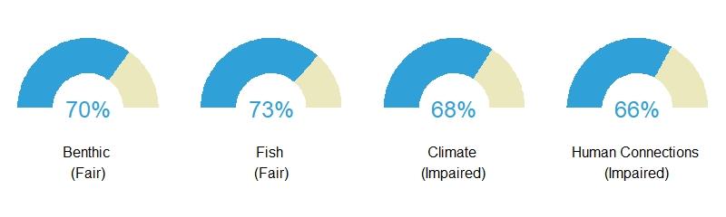
The scores you see for each region are composite scores for the themes and then one overall score. The overall score is an average of all four theme scores for the Florida region’s coral reef ecosystem score.
Benthic – Composite gauge for benthic theme score in the Florida region is 70%, meaning it is ranked fair with some indicators meeting reference values.
Fish – Composite gauge for fish theme score in the Florida region is 73%, meaning it is ranked fair with some indicators meeting reference values.
Climate – Composite gauge for climate theme score in the Florida region is 68%, meaning it is ranked impaired with very few indicators meeting reference values.
Human connections – Composite gauge for human connections theme score in the Florida region is 66%, meaning it is ranked impaired with very few indicators meeting reference values.
Overall Ecosystem – Overall coral reef ecosystem score for the Florida region is 69%, meaning it is ranked impaired with very few indicators meeting reference values.
Description of each theme is provided in the indicator information section below.
Gauge values
90–100% Very good: All or almost all indicators meet reference values.
80–89% Good: Most indicators meet reference values.
70–79% Fair: Some indicators meet reference values.
60–69% Impaired: Few indicators meet reference values.
0–59% Critical: Very few or no indicators meet reference values.
Description of Florida coral reefs
Florida’s coral reef extends from Martin County on the Atlantic Coast of Florida through the Keys to the Dry Tortugas in the Gulf of Mexico. Florida’s coral reef is the only coral reef found along the coast of the continental United States. It was divided into three sub-regions to evaluate condition. The three regions are Southeast Florida, Florida Keys, and Dry Tortugas. The Dry Tortugas encompass a small group of islands approximately 67 miles west of Key West, Florida. Most of the Dry Tortugas lie within the National Park. The total coral reef hardbottom habitat less than 30 m in depth that was monitored is 1,190 sq km.
Description of Coral Reefs:
Coral reefs are some of the most diverse and valuable ecosystems on Earth. Though they cover less than one percent of the Earth’s surface, they are estimated to provide ecosystem services (economic and environmental services) worth hundreds of billions of dollars each year. Healthy reefs protect islands and coasts from storm surge, contribute to local economies through tourism (i.e., sportfishing, snorkeling, and diving), and contribute about one-quarter of the total fish catch, providing critical food resources for tens of millions of people particularly in developing island nations.
Data Source:
The coral reef ecosystem scores shown here were analyzed using data from the National Coral Reef Monitoring Program (NCRMP). The scores you see for each region are composite scores for all four themes (benthic, fish, climate, human connections) assessed separately and then one overall score. The overall score is an average of all four theme scores for a specific region’s coral reef ecosystem score. The sources for these values and geographical regions are obtained from the NCRMP’s Status Report Scoring Methodology for Pacific Jurisdictions and 2020 Status Report Scoring Methodology for Atlantic Jurisdictions. The definitions for the themes are as follows:
- Benthic (Corals & algae): Corals and algae make up the base of the coral reef ecosystem, providing food and shelter for fish and other marine animals.
- Fish: Coral reefs serve a vital ecological role for fish species. Fish are important to the ecology of the reef, the economy, and the livelihoods of local communities.
- Climate: Climate affects all components of a reef system. Climate change and ocean acidification influence reefs across the globe, but conditions vary at the regional and local level.
- Human Connections: Coral reef management agencies protect reef resources through management plans, public education, and involving communities in managing their resources.
Southeast Overfished Stocks
Between 2020 and 2025 the number of overfished stocks shows no trend.
The x-axis represents years. The y-axis represents the number of fish stocks or fish populations that are deemed by NOAA as overfished. Overfished means the population of fish is too low. Therefore the population cannot support a large amount of fishing.
Description of time series:
The series shows the number of fish populations that have qualified as overfished since 2000. Between 2020 and 2025 the number of overfished stocks shows no trend.
Description of Overfished stocks:
An overfished stock is a population of fish that is too low. A stock that is experiencing overfishing has an annual rate of catch that is too high. Therefore the population cannot support that level of fishing and is below that level is deemed “overfished.” A fish population can be “overfished” as the result of many factors, including overfishing, as well as habitat degradation, pollution, climate change, and disease. The Magnuson-Stevens Act mandates that overfished stocks and stocks experiencing overfishing be reported annually. Stock status is determined by NOAA, based on the results of stock assessments.
Data Source:
Data were obtained from the NOAA Fisheries Fishery Stock Status website. Stocks that met the criteria for overfished status were summed by year for each region.
Close
Southeast and Gulf of America ESA
Status and Trend Analyses were not appropriate for marine mammal data.
Values Correspond to the Number of ESA Threatened or Endangered Species in a given region
Data Interpretation
Status and Trend Analyses were not appropriate for marine mammal data.
Description of Threatened and Endangered Marine Mammals (ESA):
NOAA Fisheries is responsible for the protection, conservation, and recovery of endangered and threatened marine and anadromous species under the Endangered Species Act (ESA). The ESA aims to conserve these species and the ecosystems they depend on. Under the ESA, a species is considered endangered if it is in danger of extinction throughout all or a significant portion of its range, or threatened if it is likely to become endangered in the foreseeable future throughout all or a significant portion of its range See a species directory of all the threatened and endangered marine species under NOAA Fisheries jurisdiction, including marine mammals.
Under the ESA, a species must be listed if it is threatened or endangered because of any of the following 5 factors:
1) Present or threatened destruction, modification, or curtailment of its habitat or range;
2) Over-utilization of the species for commercial, recreational, scientific, or educational purposes;
3) Disease or predation;
4) Inadequacy of existing regulatory mechanisms; and
5) Other natural or manmade factors affecting its continued existence.
The ESA requires that listing determinations be based solely on the best scientific and commercial information available; economic impacts are not considered in making species listing determinations and are prohibited under the ESA. There are two ways by which a species may come to be listed (or delisted) under the ESA:
- NOAA Fisheries receives a petition from a person or organization requesting that NOAA lists a species as threatened or endangered, reclassify a species, or delist a species.
- NOAA Fisheries voluntarily chooses to examine the status of a species by initiating a status review of a species.
Data Background and Caveats
NOAA Fisheries goes through required regulatory steps to list, reclassify, or delist a species under the ESA. For more information, see a step-by-step description of the ESA listing process. The listing process requires time and resources; as a result, the timing and number of listed marine species is not necessarily indicative of the actual number of currently endangered or threatened species and the exact timing of when these species became eligible to be listed under the ESA. Many marine species were initially listed when the ESA was passed in 1973; others have taken more time to be listed, and some have been reclassified or delisted since then.
Southeast and Gulf of America MMPA
Status and Trend Analyses were not appropriate for marine mammal data.
Values correspond to the number of MMPA Strategic or Depleted Marine Mammal Species listed each year in each region
Data Interpretation
Status and Trend Analyses were not appropriate for marine mammal data.
Description of Marine Mammal Strategic and Depleted Stocks (MMPA):
A stock is defined by the Marine Mammal Protection Act (MMPA), as a group of marine mammals of the same species or smaller taxa in a common spatial arrangement, that interbreed when mature. See a list of the marine mammal stocks NOAA protects under the MMPA.
A strategic stock is defined by the MMPA as a marine mammal stock—
- For which the level of direct human-caused mortality exceeds the potential biological removal level or PBR (defined by the MMPA as the maximum number of animals, not including natural mortalities, that may be removed from a marine mammal stock while allowing that stock to reach or maintain its optimum sustainable population);
- Which, based on the best available scientific information, is declining and is likely to be listed as a threatened species under the Endangered Species Act (ESA) within the foreseeable future; or
- Which is listed as a threatened or endangered species under the ESA, or is designated as depleted under the MMPA.
A depleted stock is defined by the MMPA as any case in which—
- The Secretary of Commerce, after consultation with the Marine Mammal Commission and the Committee of Scientific Advisors on Marine Mammals established under MMPA title II, determines that a species or population stock is below its optimum sustainable population;
- A State, to which authority for the conservation and management of a species or population stock is transferred under section 109, determines that such species or stock is below its optimum sustainable population; or
- A species or population stock is listed as an endangered species or a threatened species under the ESA.
Data Background and Caveats
NOAA Fisheries prepares marine mammal stock assessment reports to track the status of marine mammal stocks. Some marine mammal stocks are thriving, while others are declining, and we often don’t know all the reasons behind a species or stock’s population trend. Because of this variability, it is difficult to indicate the state of an ecosystem or specific region using stock assessment data for marine mammal species that often range across multiple ecosystems and regions.
Close
Southeast Marine Species Latitude
Between 2019 and 2024 the average species latitudinal shift showed no trend.
Values indicate annual cumulative change in centroid across all species in a region in degrees N
Description of Time Series: Between 2019 and 2024 the average species latitudinal shift showed no trend.
Indicator Source Information:
This data was obtained from the Distribution Mapping and Analysis Portal (DisMAP) and provides important information for fisheries management including where species are caught where and at what depth. The latitudinal (or depth) centroid is the biomass-weighted center of a population’s distribution. This metric is calculated by the DisMAP portal team using the interpolated biomass distribution surface they generated from the survey catch data, such that the latitudinal (or depth) centroids are the mean latitude (or depth) of the species distribution, where each raster cell latitude (or depth) is weighted by the value of weight-per-unit-effort for that cell. Scientists at NOAA use this data to calculate each species’ centroid as the mean latitude and depth of catch in the survey, weighted by biomass. The centroid for each species is calculated for each year after standardizing the data to ensure that the measure is consistent over time despite changes in survey techniques and total area surveyed. This data provides important information for fisheries management including which species are caught where and at what depth.
Data Background and Caveats:
The regional and national marine species distributions shown here represent the average shift in the centroid of a selected core set of species that are caught every year in surveys conducted in each region. These species represent a wide range of habitats and species types. As species distributions respond to many environmental and biological factors, combining data from multiple diverse species allows for a more complete picture of the general trends in marine species distribution. In order to more easily track and display changes in these distributions, the first year is standardized to zero. Thus, the indicator represents relative change in distribution from the first survey year.
Southeast Marine Species Depth
Between 2019 and 2024 the average species water column depth shift showed no trend.
Values Indicate annual cumulative change in average species centroid depth in meters - for example, a value of -5 indicates the species centroid moving deeper by 5m.
Description of Time Series: Between 2019 and 2024 the average species water column depth shift showed no trend.
Indicator Source Information:
This data was obtained from the Distribution Mapping and Analysis Portal (DisMAP) and provides important information for fisheries management including where species are caught where and at what depth. The metric is calculated by the DisMAP portal team using the interpolated biomass distribution surface they generated from the survey catch data, such that the latitudinal (or depth) centroids are the mean latitude (or depth) of the species distribution, where each raster cell latitude (or depth) is weighted by the value of weight-per-unit-effort for that cell. The centroid for each species is calculated for each year after standardizing the data to ensure that the measure is consistent over time despite changes in survey techniques and total area surveyed. This data provides important information for fisheries management including which species are caught where and at what depth.
Data Background and Caveats:
The regional and national marine species distributions shown here represent the average centroid of a selected core set of species that are caught every year of the surveys in a region. These species represent a wide range of habitats and species types. As species distributions respond to many environmental and biological factors, combining data from multiple diverse species allows for a more complete picture of the general trends in marine species distribution. In order to more easily track and display changes in these distributions, the first year is standardized to zero. Thus, the indicator represents relative change in distribution from the first survey year.
Southeast Forage
The data presented in this time series is South Atlantic Menhaden adults (age 1+). Due to COVID-19 no data was collected in 2020 or 2021 so there is no status or trend update.
Values correspond to catch per unit effort index score
Description of time series:
The data presented in this time series is South Atlantic Menhaden adults (age 1+). Due to COVID-19 no data was collected in 2020 or 2021 so there is no status or trend update.
Indicator information:
Forage fish or otherwise known as small pelagics are fish and invertebrates (like squids) that inhabit - the pelagic zone - the open ocean. Small pelagic species are often important to fisheries and serve as forage for commercially and recreationally important fish, as well as other ecosystem species (e.g. seabirds and marine mammals). The number and distribution of pelagic fish vary regionally, depending on multiple physical and ecological factors (i.e., the availability of light, nutrients, dissolved oxygen, temperature, salinity, predation, abundance of phytoplankton and zooplankton, etc.). Small pelagics are known to exhibit “boom and bust” cycles of abundance in response to these conditions. Examples include anchovies, sardines, shad, menhaden and the fish that feed on them.
The Southeast Atlantic forage indicator is the Menhaden CPUE Index score used by the Southeast Integrated Ecosystem Assessment team in their upcoming Ecosystem Status Report. Menhaden (Brevoortia tyrannus) are thought to play a substantial role in ecosystem structure and function. At the time of writing, the report is under review and data are not publicly available.
Data background and caveats:
Units, time series, and species vary by region for this indicator, so no national score is provided. Best practices and caveats vary by region.
No Caveats.
Southeast Ryther Index
Between 2016 and 2021, average annual Ryther Index values from the Southeast were similar to historical patterns, and there is no trend in values.
Values correspond to Ryther Index values
Data Interpretation:
Ecosystem Overfishing Time Series
Between 2016 and 2021, average annual Ryther Index values from the Southeast were similar to historical patterns, and there is no trend in values.
Indicator Source Information:
Landings are reported in tons of round (live) weight for all species or groups except univalve and bivalve mollusks, such as clams, mussels, oysters and scallops, which are reported as weight of meats (excludes shell weight). Landings data may sometimes differ from state-reported landings due to our reporting of mollusks in meat weights rather than gallons, shell weight, or bushels. Also, NMFS includes some species such as kelp and oysters that are sometimes reported by state agricultural agencies and may not be included with state fishery agency landings data.
Data Background and Caveats:
All landings summaries used in the compilation of this indicator only include non-confidential data. Federal statutes prohibit public disclosure of landings (or other information) that would allow identification of the data contributors and possibly put them at a competitive disadvantage. Most summarized landings here are non-confidential, but whenever confidential landings occur they have been combined with other landings and usually reported as "Withheld for Confidentiality" Total landings by state include confidential data and will be accurate, but landings reported by individual species may, in some instances, be misleading due to data confidentiality, which would be minimal given the aggregated nature of how these data were combined.
Landings data do not indicate the physical location of harvest but the location at which the landings either first crossed the dock or were reported from, as associated with major regions in the US
Many fishery products are gutted or otherwise processed while at sea and are landed in a product type other than round (whole) weight. Our data partners have standard conversion factors for the majority of the commonly caught species that convert their landing weights from any product type to whole weight. It is the whole weight that is displayed in our web site landing statistics. Caution should be exercised when using these statistics. An example of a potential problem is when landings statistics are used to monitor fishery quotas. In some situations, specific conversion factors may have been designated in fishery management plans or Federal rule making that differ from those historically used by NOAA Fisheries in reporting landings statistics.
Landings do not include aquaculture products except for clams, mussels and oysters.
Pacific landings summarized by state include an artificial “state” designation of “At-Sea Process, Pac.” This designation was assigned to landings consisting of primarily whiting caught in the EEZ off Washington and Oregon that were processed aboard large vessels while at sea. No Pacific state lists these fish on their trip tickets which are used to report state fishery landing, hence the at-sea processor designation was used to insure that they would be listed as a U.S. landing.
Landing summaries are compiled from data bases that overlap in time and geographic coverage, and come from both within and outside of NOAA Fisheries.
Ecosystem overfishing metrics also have potential thresholds, usually for the Ryther Index of approximately 1; but we do not report Ryther index values here relative to any threshold. Rather, we report the value of the indices for each region relative to their time series values. Comparison to some regional reports may slightly differ due to the inclusion or exclusion of specific species, but the same general trends are observed and align.
Southeast Coastal Population
The 2017 – 2022 average coastal population in the Southeast was substantially above historic levels, although the recent trend is not different from historical trends.
Values correspond to the total coastal population for a given region
Time Series
The 2017 – 2022 average coastal population in the Southeast was substantially above historic levels, although the recent trend is not different from historical trends.
Indicator Source Information:
The American Community Survey (ACS) helps local officials, community leaders, and businesses understand the changes taking place in their communities. It is the premier source for detailed population and housing information about our nation.
Data Background and Caveats:
The values represented here are coastal county population estimates for states bordering US Large Marine Ecosystems as calculated by the US Census Bureau from the American Community Survey.
Southeast Coastal Tourism GDP
Between 2016 and 2021 the average change in coastal county tourism GDP showed a significant decreasing trend.
Values correspond to percent change in the GDP of the Tourism Sector of Coastal Counties in US States that border a region
Description of Time Series: Between 2016 and 2021 the average change in coastal county tourism GDP showed a significant decreasing trend.
Indicator Source Information
Coastal tourism Gross Domestic Product is the total measure (in billions of 2012 dollars) of goods and services provided from various industries involved in tourism services and products along the coast. Data for Coastal Counties come from the US Census Bureau. This dataset represents US counties and independent cities which have at least one coastal border and select non-coastal counties and independent cities based on proximity to estuaries and other coastal counties. The dataset is built to support coastal and ocean planning and other activities pursuant to the Energy Policy Act, Coastal Zone Management Act, Magnuson-Stevens Fishery Conservation and Management Act, National Environmental Policy Act, Rivers and Harbors Act and the Submerged Lands Act.
Southeast Coastal Tourism Employment
Between 2016 and 2021 the average change in coastal county employment showed a significant decreasing trend and was below historic norms.
Values correspond to percent change in the total Employment of the Tourism Sector of Coastal Counties in US States that border a region
Description of Time Series: Between 2016 and 2021 the average change in coastal county employment showed a significant decreasing trend and was below historic norms.
Indicator Source Information:
Coastal tourism employment is the total measure of jobs in tourism industries along the coast. Data for Coastal Counties come from the US Census Bureau. This dataset represents US counties and independent cities which have at least one coastal border and select non-coastal counties and independent cities based on proximity to estuaries and other coastal counties. The dataset is built to support coastal and ocean planning and other activities pursuant to the Energy Policy Act, Coastal Zone Management Act, Magnuson-Stevens Fishery Conservation and Management Act, National Environmental Policy Act, Rivers and Harbors Act and the Submerged Lands Act.
Southeast Tourism Wage
Between 2016 and 2021 the average total coastal county real wage compensation showed a decreasing trend.
Values correspond to millions of dollars of total real wage compensation of the Tourism Sector of Coastal Counties in US States that border a region
Description of Time Series: Between 2016 and 2021 the average total coastal county real wage compensation showed a decreasing trend.
Indicator Source Information:
Coastal tourism wage is the measure of wages (nominal) paid to employees in tourism industries along the coast. Data for Coastal Counties come from the US Census Bureau. This dataset represents US counties and independent cities which have at least one coastal border and select non-coastal counties and independent cities based on proximity to estuaries and other coastal counties. The dataset is built to support coastal and ocean planning and other activities pursuant to the Energy Policy Act, Coastal Zone Management Act, Magnuson-Stevens Fishery Conservation and Management Act, National Environmental Policy Act, Rivers and Harbors Act and the Submerged Lands Act.
Southeast Total Coastal Employment
Average coastal employment within the Southeast between 2017 and 2021 was similar to historical levels, although a decreasing trend is apparent over that same period.
Values correspond to total employment in all industries in the coastal counties of a given region
Time Series
Average coastal employment within the Southeast between 2017 and 2021 was similar to historical levels, although a decreasing trend is apparent over that same period.
Data Source:
Coastal employment numbers were downloaded from the NOAA ENOW Explorer Tool, filtered to present only coastal county values using the Census Bureau’s list of coastal counties within each state. ENOW Explorer streamlines the task of obtaining and comparing economic data, both county and state, for the six sectors dependent on the ocean and Great Lakes: living resources, marine construction, marine transportation, offshore mineral resources, ship and boat building, and tourism and recreation. Data are derived from Economics: National Ocean Watch (ENOW), available on NOAA’s Digital Coast. Of note is that these data fail to include self-employed individuals. Coastal county employment numbers were then summed within each region for reporting purposes.
Southeast Commercial Landings
Between 2019 and 2024, commercial landings from the Southeast were similar to historic levels, and there is no recent trend apparent.
Values correspond to landings in millions of metric tons
Commercial Landings Time Series
Between 2019 and 2024, commercial landings from the Southeast were similar to historic levels, and there is no recent trend apparent.
Indicator Source Information:
Landings are reported in pounds of round (live) weight for all species or groups except univalve and bivalve mollusks, such as clams, mussels, oysters and scallops, which are reported as pounds of meats (excludes shell weight). Landings data may sometimes differ from state-reported landings due to our reporting of mollusks in meat weights rather than gallons, shell weight, or bushels. Also, NMFS includes some species such as kelp and oysters that are sometimes reported by state agricultural agencies and may not be included with state fishery agency landings data.
Data Background and Caveats:
All landings summaries will return only non confidential landing statistics. Federal statutes prohibit public disclosure of landings (or other information) that would allow identification of the data contributors and possibly put them at a competitive disadvantage. Most summarized landings are non confidential, but whenever confidential landings occur they have been combined with other landings and usually reported as "Withheld for Confidentiality" Total landings by state include confidential data and will be accurate, but landings reported by individual species may, in some instances, be misleading due to data confidentiality.
Landings data do not indicate the physical location of harvest but the location at which the landings either first crossed the dock or were reported from.
Many fishery products are gutted or otherwise processed while at sea and are landed in a product type other than round (whole) weight. Our data partners have standard conversion factors for the majority of the commonly caught species that convert their landing weights from any product type to whole weight. It is the whole weight that is displayed in our web site landing statistics. Caution should be exercised when using these statistics. An example of a potential problem is when landings statistics are used to monitor fishery quotas. In some situations, specific conversion factors may have been designated in fishery management plans or Federal rule making that differ from those historically used by NOAA Fisheries in reporting landings statistics.
The dollar value of the landings are ex-vessel (as paid to the fisherman at time of first sale) and are reported as nominal (current at the time of reporting) values. Users can use the Consumer Price Index (CPI) or the Producer Price Index (PPI) to convert these nominal landing values into real (deflated) values.
Landings do not include aquaculture products except for clams, mussels and oysters.
Pacific landings summarized by state include an artificial “state” designation of “At-Sea Process, Pac.” This designation was assigned to landings consisting of primarily whiting caught in the EEZ off Washington and Oregon that were processed aboard large vessels while at sea. No Pacific state lists these fish on their trip tickets which are used to report state fishery landing, hence the at-sea processor designation was used to insure that they would be listed as a U.S. landing.
Landing summaries are compiled from data bases that overlap in time and geographic coverage, and come from both within and outside of NOAA Fisheries.
Southeast Commercial Revenue
Between 2019 and 2024, average annual commercial revenue from the Southeast was not different than historical patterns, and there is an increasing trend in values.
Values correspond to real revenue is 2024 US Dollars
Commercial Revenue Time Series
Between 2019 and 2024, average annual commercial revenue from the Southeast was not different than historical patterns, and there is an increasing trend in values.
Indicator Source Information:
Landings are reported in pounds of round (live) weight for all species or groups except univalve and bivalve mollusks, such as clams, mussels, oysters and scallops, which are reported as pounds of meats (excludes shell weight). Landings data may sometimes differ from state-reported landings due to our reporting of mollusks in meat weights rather than gallons, shell weight, or bushels. Also, NMFS includes some species such as kelp and oysters that are sometimes reported by state agricultural agencies and may not be included with state fishery agency landings data.
Data Background and Caveats:
All landings summaries will return only non confidential landing statistics. Federal statutes prohibit public disclosure of landings (or other information) that would allow identification of the data contributors and possibly put them at a competitive disadvantage. Most summarized landings are non confidential, but whenever confidential landings occur they have been combined with other landings and usually reported as "Withheld for Confidentiality" Total landings by state include confidential data and will be accurate, but landings reported by individual species may, in some instances, be misleading due to data confidentiality.
Landings data do not indicate the physical location of harvest but the location at which the landings either first crossed the dock or were reported from.
Many fishery products are gutted or otherwise processed while at sea and are landed in a product type other than round (whole) weight. Our data partners have standard conversion factors for the majority of the commonly caught species that convert their landing weights from any product type to whole weight. It is the whole weight that is displayed in our web site landing statistics. Caution should be exercised when using these statistics. An example of a potential problem is when landings statistics are used to monitor fishery quotas. In some situations, specific conversion factors may have been designated in fishery management plans or Federal rule making that differ from those historically used by NOAA Fisheries in reporting landings statistics.
The dollar value of the landings are ex-vessel (as paid to the fisherman at time of first sale) and are reported as nominal (current at the time of reporting) values. Users can use the Consumer Price Index (CPI) or the Producer Price Index (PPI) to convert these nominal landing values into real (deflated) values.
Landings do not include aquaculture products except for clams, mussels and oysters.
Pacific landings summarized by state include an artificial “state” designation of “At-Sea Process, Pac.” This designation was assigned to landings consisting of primarily whiting caught in the EEZ off Washington and Oregon that were processed aboard large vessels while at sea. No Pacific state lists these fish on their trip tickets which are used to report state fishery landing, hence the at-sea processor designation was used to insure that they would be listed as a U.S. landing.
Landing summaries are compiled from data bases that overlap in time and geographic coverage, and come from both within and outside of NOAA Fisheries.
Southeast Recreational Effort
Between 2019 and 2024, recreational fishing effort in Southeast is around historic levels and shows no trend.
Values correspond to cumulative number of angler trips
Description of time series:
Between 2019 and 2024, recreational fishing effort in Southeast is around historic levels and shows no trend.
Indicator Source Information
Recreational harvest and effort data pulled from National Summary Query. Units of data are in Effort in Angler Trips and Harvest in numbers of fish.The data from these queries is used by state, regional and federal fisheries scientists and managers to maintain healthy and sustainable fish stocks.
Data Background and Caveats:
To properly interpret this information, it is important to consider the following key points:
- When comparing harvest estimates across an extended time series, note differences in sampling coverage through the years. Some estimates may not be comparable over long time series.
- Changes may occur between preliminary and final estimates and year to year, meaning that the data may change when updated. Please review the Limitations and other sections on the Using the Data page from the source for more information.
Southeast Recreational Harvest
Between 2019 and 2024, recreational harvest from Southeast are around historic levels. There is no significant trend apparent.
Values correspond to harvest in millions of fish
Description of time series:
Between 2019 and 2024, recreational harvest from Southeast are around historic levels. There is no significant trend apparent.
Indicator Source Information
Recreational harvest and effort data pulled from National Summary Query. Units of data are in Effort in Angler Trips and Harvest in numbers of fish.The data from these queries is used by state, regional and federal fisheries scientists and managers to maintain healthy and sustainable fish stocks.
Data Background and Caveats:
To properly interpret this information, it is important to consider the following key points:
- When comparing catch estimates across an extended time series, note differences in sampling coverage through the years. Some estimates may not be comparable over long time series.
- Changes may occur between preliminary and final estimates and year to year, meaning that the data may change when updated. Please review the Limitations and other sections on the Using the Data page from the source for more information.
Southeast Commercial Fishing Engagement
Between 2016 and 2021 the percent of communities moderately or highly engaged in commercial fishing showed a downward trend, with 2019 presenting a series low level.
The x-axis on this time series represents years and the y-axis represents the percent of communities that are moderate to highly engaged in commercial fishing across the Southeast. Commercial fishing engagement is measured by the number permits, fish dealers, and vessel landings across coastal communities in the Southeast.
Description of time series:
This time series shows the percent of communities moderately or highly engaged in commercial fishing in Southeast from 2009 to 2021. Between 2016 and 2021 the percent of communities moderately or highly engaged in commercial fishing showed a downward trend, with 2019 presenting a series low level.
Description of Southeast Commercial Fishing Engagement:
Commercial fishing engagement is measured by the presence of fishing activity in coastal communities. The commercial engagement index is measured through permits, fish dealers, and vessel landings. A high rank within these indicates more engagement in fisheries. For details on both data sources and indicator development, please see https://www.fisheries.noaa.gov/national/socioeconomics/social-indicator….
NOAA Monitors commercial fishing engagement to better understand the social and economic impacts of fishing policies and regulations on our nation’s vital fishing communities. This and other social indicators help assess a coastal community’s resilience. NOAA works with state and local partners to monitor these indicators. We present data from the Northeast, Southeast, Gulf of Mexico, California Current, Alaska, and Hawaiian Island regions.
Data Source:
Commercial fishing engagement data is from the National Marine Fisheries Service’s social indicator data portal:https://www.st.nmfs.noaa.gov/data-and-tools/social-indicators/ The percentage of all communities in each region classified as medium, medium high, or highly engaged is presented for both recreational and commercial fishing.
Southeast Recreational Fishing Engagement
Between 2016 and 2021 the percent of communities moderately or highly engaged in recreational fishing showed a significant increasing trend.
The x-axis on this time series represents years and the y-axis represents the percent of communities that are moderately to highly engaged in recreational fishing across the Southeast US.
Recreational Engagement Time Series
This time series shows the percent of communities moderately to highly engaged in recreational fishing in the Southeast US from 2009 to 2021. Between 2016 and 2021 the percent of communities moderately or highly engaged in recreational fishing showed a significant increasing trend.
Indicator Source Information:
The Southeast recreational engagement index is measured using shore, private vessel and for-hire vessel fishing activity estimates.
Data Source:
Commercial fishing engagement data is from the National Marine Fisheries Service’s social indicator data portal:https://www.st.nmfs.noaa.gov/data-and-tools/social-indicators/ The percentage of all communities in each region classified as medium, medium high, or highly engaged is presented for both recreational and commercial fishing
Close
Southeast Billion Dollar Disasters
The number of disasters over the past 5 years is substantially higher than historical levels of events, and there is an upward trend in the number of events.
Values correspond to the number of events in a given year
Time Series
The number of billion dollar disasters within the Southeast is variable over time. The number of disasters over the past 5 years is substantially higher than historical levels of events, and there is an upward trend in the number of events.
Indicator Source Information:
Billion dollar disaster event frequency data are taken from NOAA’s National Centers for Environmental Information. The number of disasters within each region were summed for every year of available data. Although the number is the count of unique disaster events within a region, the same disaster can impact multiple regions, meaning a sum across regions will overestimate the unique number of disasters.
Data Background and Caveats:
Events are included if they are estimated to cause more than one billion U.S. dollars in direct losses. The cost estimates of these events are adjusted for inflation using the Consumer Price Index (CPI) and are based on costs documented in several Federal and private-sector databases.
Southeast Beach Closures
During the last five years, there has been no trend and values were between the 10th and the 90th percentiles of all observed data in the time series.
Beach closures are the number of days when beach water quality is determined to be unsafe.
Data Interpretation:
Time series: This time series shows the average number of beach closure days in the Southeast US region from 2000 to 2024. During the last five years, there has been no trend and values were between the 10th and the 90th percentiles of all observed data in the time series.
Indicator and source information:
Unsafe water quality may have significant impacts on human health, local economies, and the ecosystem. Beach water quality is determined by the concentration of bacteria in the water (either Enterococcus sp. or Escherichia coli).
The US Environmental Protection Agency (EPA) supports coastal states, counties and tribes in monitoring beach water quality, and notifying the public when beaches must be closed. The information presented is from states, counties, and tribes that submit data to the EPA Beach Program reporting database (BEACON). Data obtained from the EPA BEACON 2.0 website have been provided to EPA by the coastal and Great Lakes states, tribes and territories that receive grants under the BEACH Act. Data were refined to closure, by state or territory, by year.
Data background and limitations:
Data compiled by states or territories are combined in regions defined as US Large Marine Ecosystems (LME). Changes in the number of beach closure days may be driven by changes in the number of beaches monitored under the BEACH Act versus by state and local municipalities and not by changes in water and/or air quality. Not all US beach closures are captured in this database, because not all beaches in a state or territory are monitored through the EPA BEACH Act. Data that were not identified to a water body or identified as inland water were not included. Data for beaches monitored by state and local municipalities are not included.
Data from 2020 may be inflated by the Covid-19 pandemic, as there was no consistent way for states to report pandemic-related closures
Close

Florida Keys National Marine Sanctuary Condition Report
This "condition report" provides a summary of resources in the National Oceanic and Atmospheric Administration's Florida Keys National Marine Sanctuary (sanctuary), pressures on those resources, current conditions and trends, and management responses to the pressures that threaten the integrity of the marine environment.

Florida Keys National Marine Sanctuary Ecosystem Tracking Tool
This interactive graphic allows you to find data used to track the changing conditions of natural resources and levels of human use in the Florida Keys. Called “indicators,” you can hover over each icon, or click the indicator from the menu on the right to learn more about it and see the data. This is a product of the Florida Keys NOAA Integrated Ecosystem Assessment program.

Gray's Reef National Marine Sanctuary Condition Report
This “condition report” provides a summary of resources in the National Oceanic and Atmospheric Administration’s Gray’s Reef National Marine Sanctuary, pressures on those resources, current condition and trends, and management responses to the pressures that threaten the integrity of the marine environment.

MBON and the Sanctuaries MBON project
The Marine Biodiversity Observation Network (MBON) is a growing global initiative composed of regional networks of scientists, resource managers, and end-users working to integrate data from existing long-term programs to improve our understanding of changes and connections between marine biodiversity and ecosystem functions.

Southeast Coastal Ocean Observing Regional Association
SECOORA – Southeast Coastal Ocean Observing Regional Association – is the coastal ocean observing system for the Southeast U.S.
Our mission is to observe, understand, and increase awareness of our coastal ocean; promoting knowledge, economic and environmental health through strong regional partnerships.

NOAA Environmental Response Management Application (ERMA): Regional Portals
The Environmental Response Management Application is a web-based Geographic Information System (GIS) tool that assists emergency responders and environmental resource managers in dealing with incidents that may adversely impact the environment.
South Florida Marine Biodiversity Observation Network
This project will build on the foundations laid by the present Sanctuaries MBON demonstration. A close partnership with NOAA AOML and the FKNMS has focused on periodic MBON surveys of the Florida Keys since 2014. Additional partners now add animal tracking and other dimensions to the Sanctuaries MBON. Specifically, we seek to integrate ground and satellite observations related to biodiversity to inform ecosystem-based management in and around the Florida Keys National Marine Sanctuary (FKNMS).

Biscayne Bay Habitat Focus Area
Biscayne Bay is a shallow, clear water bay centered within the large metropolitan area of Miami on Florida’s lower southeast coast. The Biscayne Bay Habitat Focus Area extends nearly 50 miles from northern Dumfoundling Bay to southern Barnes Sound and Manatee Bay. It also includes the coral reef tract that runs parallel to the bay, extending northward from the Florida Keys. Biscayne Bay and its reef support an astonishing array of marine species and are favorite destinations for recreational pursuits such as fishing, boating, kayaking, snorkeling, swimming, and diving. Biscayne Bay is an iconic setting for a growing international urban center, and many community activities take place on its waters.

Middle Peninsula Habitat Focus Area
The Middle Peninsula of Virginia—surrounded by the tidal portions of the York River, the Piankatank River, and Mobjack Bay—is a landscape of scattered farms, forests, and small rural towns. It is known for its recreational opportunities, maritime industries, and indigenous and colonial-era history. The waters contain rich beds of submerged aquatic vegetation that support important commercial and recreational fisheries such as bluefish, summer flounder, and black sea bass, along with endangered Atlantic sturgeon. Oyster reefs, although substantially reduced from historic numbers, are being restored in rivers throughout the region. However, this rural area is experiencing significant impacts driven by climate change.

NOAA Digital Coast
The Digital Coast was developed to meet the unique needs of the coastal management community. The website provides not only coastal data, but also the tools, training, and information needed to make these data truly useful. Content comes from many sources, all of which are vetted by NOAA.
Data sets range from economic data to satellite imagery. The site contains visualization tools, predictive tools, and tools that make data easier to find and use. Training courses are available online or can be brought to the user’s location. Information is also organized by focus area or topic.
NOAA Southeast and Caribbean Region
From the Carolinas to the Florida Keys and the U.S. Caribbean, NOAA has substantial capabilities working to address priorities and needs of our stakeholders and partners in the Southeast and Caribbean Region. Several NOAA centers, offices, and laboratories serve this region, with workforce concentrations in Beaufort, NC; Asheville, NC; Charleston, SC; St. Petersburg, FL; Miami, FL; and Key West, FL. The region also boasts three National Marine Sanctuaries, one River Forecast Center, a Tsunami Warning Program and Seismic Network, Weather Forecast Offices in all southeastern states and the U.S. Caribbean, and the National Hurricane Center.
DisMAP
DisMAP provides access to distribution information for more than 800 marine species caught in NOAA Fisheries bottom trawl surveys in five regions in the United States (Northeast, Southeast, Gulf of Mexico, West Coast, and Alaska). In this first version of the portal all species distribution products are derived from NOAA Fisheries regional bottom trawl survey data. They do not take into account alternative sources of fisheries data such as long-line, plankton, video, or fishery-dependent surveys. Because of this, distribution products are not available for the Pacific Islands or Caribbean regions at this time as those regions do not have bottom-trawl surveys; however incorporating these additional data sources is an area of interest for future releases.
